Mathematics for Class XI - Limits

Dear Children,

The link below gives a simplified explanation to the concept of 'Limits' and is meant for Class XI Math Students.

https://www.mathsisfun.com/calculus/limits.html

Do share with me what you learnt from it and how you found it.

Tanvi Ma'am

Short Stories by O'Henry

This post is meant especially for the students of Class VIII

Dear Children ,
We have enjoyed reading short stories for some time now. Here, in this post, you will find the short stories of O'Henry uploaded for your convenience, in case some of you haven't yet had the opportunity to read his works.

https://drive.google.com/file/d/0B8_xRbscAKFjWVhpUFlVbXg0c2c/view?usp=sharing

Do Not Go Gentle into That Good Night by Dylan Thomas

This post is specifically meant for Class XI.

We have just read 'Do Not Go Gentle into That Good Night by Dylan Thomas' . This poem made familiar by the recent movie 'Interstellar' was not so difficult to understand. However, there is a lot more we can learn about Dylan Thomas himself that will help us develop a perspective of our own when we read the poem again.

So- here is a little about Dylan Thomas. Courtesy http://www.bbc.co.uk/schools/primaryhistory/famouspeople/dylan_thomas/ 

(You will also find an interestingly put up timeline that tells us all about his life here and if you would like to view his works , you could do so here . )

Dylan Thomas. Born in 1914 at the start of World War I Dylan Thomas grew up to be a famous Welsh poet best known for his work Under Milk Wood, Do Not Go Gentle into the Good Night and A Child's Christmas. He was only 21 when he became the leading Anglo-Welsh poet of his time. In his poems, Dylan Thomas used words in fresh and exciting ways. He loved the sounds of words, so his poems are great for reading aloud. He wrote about his life, his friends, and about Wales. Some poems are serious, some are funny.

Catch a glimpse of the house where Dylan Thomas was born and lived until his parents moved out in 1937.This was the "…Glamorgan villa…" overlooking the "…long and splendid curving shore…" of Swansea Bay. This is where the subject of the film Edge of Love and author of Under Milk Wood spent his formative years. Dylan's birthplace has now been fully restored to its condition in 1914 when it was bought as a new house by the Thomas family.

Dylan Marlais Thomas was born in Wales on 27 October 1914. His father David John ('DJ') Thomas was an English teacher at Swansea Grammar School. His mother, Florence Williams, was a seamstress, but gave up work to look after her children. The Thomas family had a maid to help with housework.
Dylan's sister, Nancy, was 8 when Dylan was born. The family lived at 5 Cwmdonkin Drive, Swansea. Dylan had several aunts and uncles in the town. Florence spoiled her curly-headed son. If he said he felt ill, she let him off school.
'DJ' and Florence spoke Welsh, but Dylan spoke only English. The first poems he remembered were nursery rhymes. He loved the sounds of words.
Dylan started writing poems when he was 8. In 1925 he went to Swansea Grammar School. His first poem soon appeared in the school magazine. His father was in charge of the magazine!
At school, Dylan was good at English, but sometimes badly behaved. Most of all, he loved writing poetry. In 1927, he got paid for a poem by the Western Mail newspaper.
In 1930 Dylan sent some poems to Robert Graves, a famous poet. Graves liked them. Dylan was encouraged, and wrote many poems while still a teenager.
In 1931 Dylan left school. He got a job as a reporter on the South Wales Evening Post newspaper. He left next year but went on writing reviews of plays and concerts. Dylan enjoyed acting, though other actors were upset if he wrote rude things about them!
Dylan met his friends in a Swansea café, or in a pub. He loved to talk, tell stories, and read his poems aloud. He said poems should be read 'by the ears' and not just 'by the eyes'.
In 1933 he visited London for the first time. First he stayed with his sister and her husband. Then he shared rooms with friends. London was much bigger than Swansea. It was exciting to be in a city with so many writers and artists.
Life as a poet
In 1934 Dylan Thomas published his first book of poems, called 18 Poems. He was becoming known as a young poet. More people read his poems, liking how he used words, and how he wrote about Wales.
In 1936, Dylan met Caitlin Macnamara, a dancer. She knew lots of writers and artists. Dylan and Caitlin were married in July 1937.
In 1938 Dylan and Caitlin moved to the small town of Laugharne, in South Wales. Their house was called 'Sea View'. In 1939, their son Llewelyn was born.
In September 1939 World War II began. Dylan was not well enough to be a soldier. When called for army interview, he went into the room looking so ill he was excused. With paper rationed, many publishing firms closed. It was hard to make money from writing. In 1943 Dylan and Caitlin had a daughter, Aeronwy. Times were hard.
During World War II, Dylan wrote scripts for films and for the BBC. The war ended in 1945. Dylan broadcast on BBC Children's Hour about 'Memories of Christmas'. He was writing some of his best poems too.
In 1949 Dylan and Caitlin moved back to Laugharne. Their son Colm was born, but Dylan and Caitlin had many quarrels.
In 1950, Dylan went to America to read his poems and talk to students. He did not like America much. When he met film star Charlie Chaplin, he drove a car across the tennis court!
In 1952 his Collected Poems were published. Dylan's parents also lived in Laugharne. When Dylan's father became ill Dylan wrote a poem to encourage him to get better, Do Not Go Gentle Into That Good Night. It is one of Dylan's most famous poems, it was also one of his last.
In 1953 Dylan went to America for the third time. He arrived just before his 39th birthday. He became very ill.
He enjoyed holidays on his Aunt Ann's farm in Carmarthenshire. Dylan's mother helped him read, and gave him comics. His father read Shakespeare to him.
In 1937 Dylan Thomas made his first radio broadcast, for BBC Wales. He talked about poetry.
Some of Dylan's poems were published in America. He wrote about growing up in stories called Portrait of the Artist as a Young Dog.
Their home, The Boat House, is now a Dylan Thomas museum. Dylan wrote in an old shed. He spent most evenings in the town's hotel, with his friends.
Dylan Thomas died in a New York hospital on 9 November 1953.

Find an analysis of the poem Do Not Go Gentle...in the video below.

The poem is structured as a villanelle with a set rhyme scheme but no well-organised meter or fixed number of syllables. A Villanelle is divided into three segments. The first segment is called the introduction. The second is called the development and the third is called the conclusion.

Here is a reading of the poem by the man himself.

And here, you could watch a biography on the poet.

Here is a link to an article that was published about the rock-and-roll poet, Dylan Thomas to mark his centenary last year. http://www.bbc.com/culture/story/20141016-dylan-thomas-rock-n-roll-poet

Here's another line by line analysis for you to read http://genius.com/Dylan-thomas-do-not-go-gentle-into-that-good-night-annotated

Museum of Mathematics!

We always associate a museum with History or anything related to it. But Math? Seriously. It came as a pleasant surprise to discover that there really is a Museum of Mathematics in New York.

You will find out more about it here.

Exciting, isn't it?

Evidence of Water on Mars!!!

Talk about timing! While NASA approved movie 'The Martian' gets ready to premiere on Friday, Scientists at NASA have, in reality , confirmed the evidence of water on Mars.  Liquid water is essential to life and the possibility of microscopic life forms in a neighbour planet is indeed overwhelmingly exciting.

Well, Children, although the internet is teeming with news of this confirmation , you can also find out all about it here.  We've lined up a video clip and some links to tell you a little more about the significance of this discovery.
Don't forget to discuss it with your teachers , family and friends.

 Click here to read news about Water on Mars 

Click here to read news about  NASA's discovery of water on Mars.

Here's what the New York Times says about it

And here, The Indian Express sums it up quite beautifully.

 http://www.reuters.com/  video/2015/09/28/evidence-of-recent-water-flows-on-mars-s?videoId=365753905

The Highwayman- Alfred Noyes

Reposting the article from an earlier blog - written for my students back in 2013
These days understanding literature has become so much easier what with the internet's humongous repertoire. But then, you need to analyse every detail you read for not everything up there on the net will be true although it may be someone's point of view put across rather strongly.

Recently , when I read 'The Highwayman' trying to identify the threads of poetic craft that ran through it, the very experience of reading this poem filled me with wonder. Wonder at how the poet could have taken a not-so-heroic highway robber and simply with the help of well-crafted phrases and a thrilling romantic plot turn around our perception of the highwayman. So our sympathies lie, not with the law, not with what history tells us about highwaymen of the 18th century, but with the young, dashing highwayman who is hopelessly in love with Bess, the landlord's daughter, the man who promises to be back to his beloved , the courageous young lover who comes riding back to seek revenge for his lady love's death, only to die a dog's death himself. He has been betrayed by the jealous ostler Tim, who had overheard him parting ways with Bess. Tim, whose description makes it obvious that he is hardly our choice of a hero, is also in love with Bess but knows he cannot get her as Bess's heart has already been won by the highwayman.

When the Highwayman enters the scene - the fact that he is riding is emphasized by the repetition- that is what he chiefly does, rides down the highway. Noyes describes the highwayman's appearance quite meticulously right from the French cocked hat, the wine red coat to his brown breeches and laced up chin, his boots, his pistol, his rapier.

We see him being described again later in the poem, but this time he is in wild rage, as the news of Bess's tragic death has reached him.

The dark and windy night sky is painted vividly in striking metaphorical language

'The wind was a torrent of darkness among the gusty trees.  

The moon was a ghostly galleon tossed upon cloudy seas.  

The road was a ribbon of moonlight over the purple moor...'

In the dark of the night does all the action take place. The moonlight is ghostly, shadowy - hardly able to survive the clouds- like a ship being tossed about by the waves in the sea.The setting foreshadows the tragic events that are to happen soon.

One more character that stays with us is Bess. She gives up her life for the man she loved. True love for years has been elevated to fame with the death of lovers. But in this poem the lovers meet, although it is  after their death. For even now in the moonlight one can hear the highwayman come riding, riding, riding...

I enjoyed my experience of reading The Highwayman thoroughly and am sure all my students who read it with me did.

Here are some links that I chanced upon while looking up the poem.

<ahref="http://www.bbc.co.uk/wales/mid/halloffame/arts/alfrednoyes.shtml">http://www.bbc.co.uk/wales/mid/halloffame/arts/alfrednoyes.shtml

http://en.wikipedia.org/wiki/The_Highwayman_(poem)

http://www.localhistories.org/highwaymen.html

http://bluegatefieldsjuniors.co.uk/The%20Highwayman%20yr5.pdf

Amazing song by Loreena McKennit - The Highwayman - although some parts are missing-

http://www.youtube.com/watch?v=UvKBPr71dhA

Grammar Test

For the following grammar test you give yourself for practice - you are supposed to complete this in 20 minutes. Can you do it and manage to ace it as well? Try it! You may set yourself marks for this on your own... :)

Question 1

You must do as you have been directed in the brackets...

i.  Sona bit into a delicious chocolate cake. [Begin: The cake…]

ii.  Rajiv failed to score high marks in the test. [Change into a negative sentence]

iii. Being innocent, my little brother does everything he is asked to do if we call him 'superhero'.

[ Use; so…. that]

iv. Preeti ought not to have hidden the picture when she found it. ( It was wrong...)

v. As soon as the I reached the bus stop, everyone crowded around me. [Begin: No sooner…..]

vi. “You need to have breakfast everyday or else you won't be able to concentrate for long.” My class 

teacher said. [Change into indirect speech]

vii. This is the best novel I have ever read. [Begin: Never…]

viii. Sheetal painted a  beautiful portrait of her aunt. [Change the voice]

Question 2

Use appropriate words  to complete the sentences given

i.  The doctors at Red Cross discovered a drug to cure him ______________ the rare disease.

ii.  I am certain the Director will disapprove __________ our decision.

iii. Do you think you will benefit ___________ my advice?    

iv.  We all can distinguish true praise _________ flattery.

v. Rajan find it difficult to be attentive_______________ what is being taught.

Question 3

Use an appropriate form of the verb given ....any tense you think suits the sentence

i. If he …………….. (has) the money , he would buy it now.

ii. A man of high principles never …………………..(break) his word.

iii. I shall be very surprised if it …………………….(rain) any more.

iv. If I had ………………………….(know) you were coming, I would have baked a cake.

Agree or Disagree?

We have disagreements all the time in real life. So it is with grammar too!

What we call rules can easily be remembered if we think of the words as behaving exactly like us, humans. They are close friends with some and at loggerheads with others.

Thus we come to that slippery subject Subject - Verb Agreement which often slips in unnoticed in many an English Language test paper and leaves us ruffled.

Let's get the facts clear first-

What is subject - verb agreement?

Take the example of ...

Shirin goes to school with her sister.

The subject in this sentence is Shirin as we are talking about Shirin in this sentence.

The verb is 'goes' since the subject is singular.

If the subject had been Shirin and her sister, then we would have to use the verb 'go', and the sentence would have been written as follows:-

Shirin and her sister go to school.

So the verb in a sentence has to agree with the subject.

Let's see if we can do the following Subject - Verb exercise. Warning: These are real tricky ones!

Fill in the blanks with an appropriate verb

( Clue:Go for the subject right next to the verb. The verb agrees with it.)

i) There _________ a cupboard and a bed in this room.

ii) Either the writers or the publisher _____________ to blame.

iii) The minister and the painter ______________ coming.

iv) The team __________ done a good job.

v)  The pair of scissors ___________ on the desk.

vi) The committee _____________ working on  the issue.

vii) Neither the students nor the teacher _____________ enjoying the show.

viii) Neither the students nor the teachers ___________ enjoying the show.

ix) Which of those charts ______________ yours?

x) The costume with all its accessories _______________ reached the salon.

useful links: http://www.towson.edu/ows/sub-verb.htm

http://grammar.ccc.commnet.edu/grammar/sv_agr.htm

http://www.icseenglishhelp.org/2008/11/prasal-verbs.html

Answers:

i) There __is___a cupboard and a bed in this room. ( We consider each of the things - hence singular- cupboard and bed)

ii) Either the writers or the publisher ___is____ to blame.( We consider the subject right next to the verb.)

iii) The minister and the painter ____are____ coming. (Here, the minister and the painter are two different people - if they are the same we use 'is')

iv) The team ____has____ done a good job. ( the team is considered to be singular as it is a collective)

v)  The pair of trousers __are___ on the bed.( The pair is considered as plural - so we use are)

vi) The committee ___is___ working on  the issue. (The committee acts as one unit - so we use the singular verb)

vii) Neither the students nor the teacher ____is_____enjoying the show.

viii) Neither the students nor the teachers ____are____ enjoying the show.

ix) Which of those charts ___is____yours? ( Which refers to a singular subject)

x) The costume with all its accessories _____has____ reached the salon.( The costume is the main subject and is singular)

The thumb rule to follow is - check whether the subject is singular or plural - then proceed.

Phenomenal Woman- Dr.Maya Angelou

To think that someone who has been through so much in life can be so positive that she inspired people across the globe, not only as long as she lived but now even after she's passed away. Truly a phenomenal woman!

Really, what a wonderfully thought - provoking poem have we read together, Class XI! I hope you've been prodded to read more about Dr. Maya Angelou after reading it.

Here, for you is the poem recited by none other than the poet herself. Listen and enjoy!

To understand the kind of person she was - even just a bit you must listen to what she has to say about humane qualities that exist in all of us. 'I am a Human Being!' She reaffirms.

If you want to take a walk through her life, listening to what she has spoken to millions the world over about,  watch this documentary that speaks volumes about her-

If you would like to know a little more about her, here's a film that takes you back in time.

Angelou speaks about her childhood in this video.

Do listen to these and let us share in class what more you have found out about Maya Angelou . What did you find fascinating about her life and her work?

You can read a lot about her - there's a host of material all over the internet. This particular article- http://www.courier-journal.com/story/opinion/readers/2014/06/04/maya-angelou-phenomenal-woman-indeed/9950061/ was written when she passed away last year.

The Last Ride Together presentation

Speaking Skills Matter!!!

Dear Children,

Experience good debates, speeches and train yourself , sharpen your reasoning and speaking skills. Listen well  and tell us what you think.

/http://www.bbc.co.uk/bitesize/ks3/english/speaking_listening/speaking/activity/ ( Absolutely amazing!)


Annapurna Ma'am

Will You Sign Up?

Dear Children,

A message from Madhu Ma'am for you:-

Here's the link to a petition to save the Aravallis in Haryana and the Mangar Bani, a magnificent locally protected Sacred Grove which has been sold off and threatened.

https://www.change.org/p/hon-ble-chief-minister-government-of-haryana-protect-the-haryana-aravalli-hills-and-forests-permanently-for-future-generations-make-gurgaon-and-faridabad-ecologically-smart-cities

These are the steps to follow in order to sign up:-

1. Click on the link
2. Click on the sign button
3. Enter name , email id and pincode
4. Submit
Do your bit if you believe in it.
Your signature can make a difference.
Thank you!

The CLABIL Summer Project

Dear Children,
Hope you have begun recording for the CLABIL Project.

India's biggest audio library in Indian languages - the Central Library of Audio Books in Indian Languages or CLABIL for short, is a boon for people who aren't blessed with the gift of eyesight. There are scores of blind people in our country and elsewhere who need to access resources the same way as we do. Having these resources in an audio format is the best thing that could happen. When we click for information on the internet and find it easily on wikipedia or other such informative sites, little do we realise how ill equipped our systems are to help the visually challenged people.

When you record an article, a story or a poem of your choice - keep that young blind student in mind- who would also like to know more , do a little bit of research or perhaps listen to another story written by a famous author. Choose a topic you would love to read out aloud- read clearly, audibly and make a connect with those who will find your voice among thousands and benefit from a few minutes of your time.

Have a great time reading and recording!

Check out the recording already present on CLABIL here - http://www.braillecards.org/audio.php

Math Mags

Children - this one is sheer fun-

A link to some Mathematics e-magazines for you to devour. Amazing, isn't it? It is rare to find magazines on Mathematics alone. So this one should be a treat for all Math lovers.

http://azimpremjifoundation.org/content/right-angles

Regards,
Tanvi & Renu Ma'am

Getting Mathematical!

Dear Children,
Here is some material on Mathematics - Geogebra . We are grateful to Dr. Jonaki B Ghosh for sharing it with us.

Hope you find this useful as well as interesting. Do share your feedback with us.

- Tanvi Ma'am and Renu Ma'am

                                                                 

            

Compiled by

Dr. Jonaki B Ghosh

Department of Elementary Education

Lady Shri Ram College for Women

Introduction

Background Information about GeoGebra

GeoGebra is dynamic mathematics software for schools that joins geometry, algebra, and calculus. It is developed for learning and teaching mathematics in schools by Markus Hohenwarter and an international team of programmers.

Multiple Views for Mathematical Objects

GeoGebra provides three different views of mathematical objects: a Graphics View, a numeric Algebra View, and a Spreadsheet View. They allow you to display mathematical objects in three different representations: graphically (e. g., points, function, graphs), algebraically (e. g., coordinates of points, equations), and in spreadsheet cells. Thereby, all representations of the same object are linked dynamically and adapt automatically to changes made to any of the representations, no matter how they were initially created.

On the one hand you can operate the provided geometry tools with the mouse in order to create geometric constructions on the drawing pad of the graphics window. On the other hand, you can directly enter algebraic input, commands, and functions into the input field by using the keyboard. While the graphical representation of all objects is displayed in the graphics window, their algebraic numeric representation is shown in the algebra window.

Basic Use of Tools

• Activate a tool by clicking on the button showing the corresponding icon.
• Open a toolbox by clicking on the lower part of a button and select another tool from this toolbox. Hint: You don’t have to open the toolbox every time you want to select a tool. If the icon of the desired tool is already shown on the button it can be activated directly. Hint: Toolboxes contain similar tools or tools that generate the same type of new object.
• Check the toolbar help in order to find out which tool is currently activated and how to operate it.

Constructing an Equilateral Triangle

Instructions

	1) We will not need the Algebra window and the Coordinate axes so we will hide them. To hide the Coordinate axes, click the View menu on the menu bar, and then click Axes. To hide the Algebra window, click View then click Algebra window.
	2) Click the Segment between two points tool, and click two distinct places on the drawing pad to construct segment AB.
	3)  If the labels of the points are not displayed, click the Move button, right click each point and click Show label from the context menu. (The context menu is the pop-up menu that appears when you right click an object.)
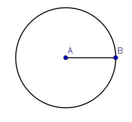
	4) To construct a circle with center A passing through B, click the Circle with Center through Point tool, click point A, and then click point B. After step 4, your drawing should look like the one shown in Figure 1. Figure 1 - Circle with center A and passing through B.
	5) To construct another circle with center B passing through A, with the Circle with Center though Point still active, click point B and then click point A
	6) Next, we have to intersect the circles. To intersect the two circles, select Intersect Two Objects, then click the circumference of both circles. Notice that two points will appear in their intersections. After step 6, drawing should look like the one shown in Figure 2.
	Figure 2 - Circles with radius AB and intersection C and D.
	7) We only need three points, points A, B and C, to form an equilateral triangle, so we will hide the two circles, segment AB and point D. To do this, right click each object and click the Show Object option to uncheck it. In hiding segment AB, be sure that you do not click points A or B.
	8) With only three points remaining on the drawing pad, click the Polygon tool and click the points in the following order: point A, point B, point C and then point A to close the polygon. After step 8, your drawing should look like the figure below. Figure 3 - Triangle formed from radii of two circles
	9)  You have probably observed that it seems that ABC is an equilateral triangle. In fact, it is. To verify, we can display the interior angles of the triangle. To do this, click the Angle tool, then click the interior of the triangle.
	10)  What do you observe? Move the vertices of the triangle. Is your observation still the same?
	11)  You can also verify the length of the sides using the Properties window. To do this, right click one of the sides of the triangle, click Object Properties from the context menu.
	12)  In the Object Properties window, select the Basic tab. Be sure that the Show label check box is checked and choose Value from the Show label drop down list.
	13) Select the other sides of the triangle in the Object list located at the left side of the Object Properties window and change the labels to Value, then close the window when you are done.

Sum of the exterior angles of a Polygon

Instructions

	1) Open GeoGebra. We will not need the Coordinate axes so we will hide them. To hide the Coordinate axes, click the View menu on the menu bar, and then click Axes.
	2) In the input bar enter n=0.01.Click on the value in the algebraic view and click on Show Object.
	3) Right click on the slider to adjust the value of n .Select Interval from0.01 to 10 with increment 0.01.Drag the slider to show value of n as 1.
	4) In Options Menu , select Labeling-New Points Only
	5) Mark a point A on the drawing pad using the point tool.
	6) Construct a circle with centre at A and radius n by using Circle with centre and radius tool.
	7) Mark a point B on the circle.
	8) Construct a regular polygon of 9 sides by selecting the Regular Polygon tool. Click on A and then B and enter 9 for Points.
	9) Right click on the circle with the Move arrow and de-select the Show Object to hide the circle.
	10) Construct Rays with one starting point as one of the vertices and other point as the adjacent vertex.
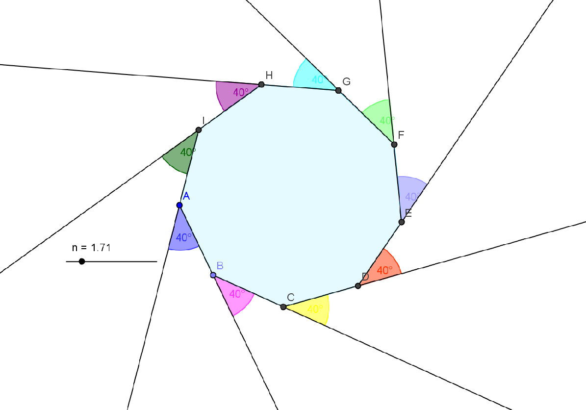
	11) Construct 9 exterior angles between the rays by selecting the angle tool and then clicking on the two rays.
	12) You can change the display of each angle by right clicking on each angle and going to Object Properties.
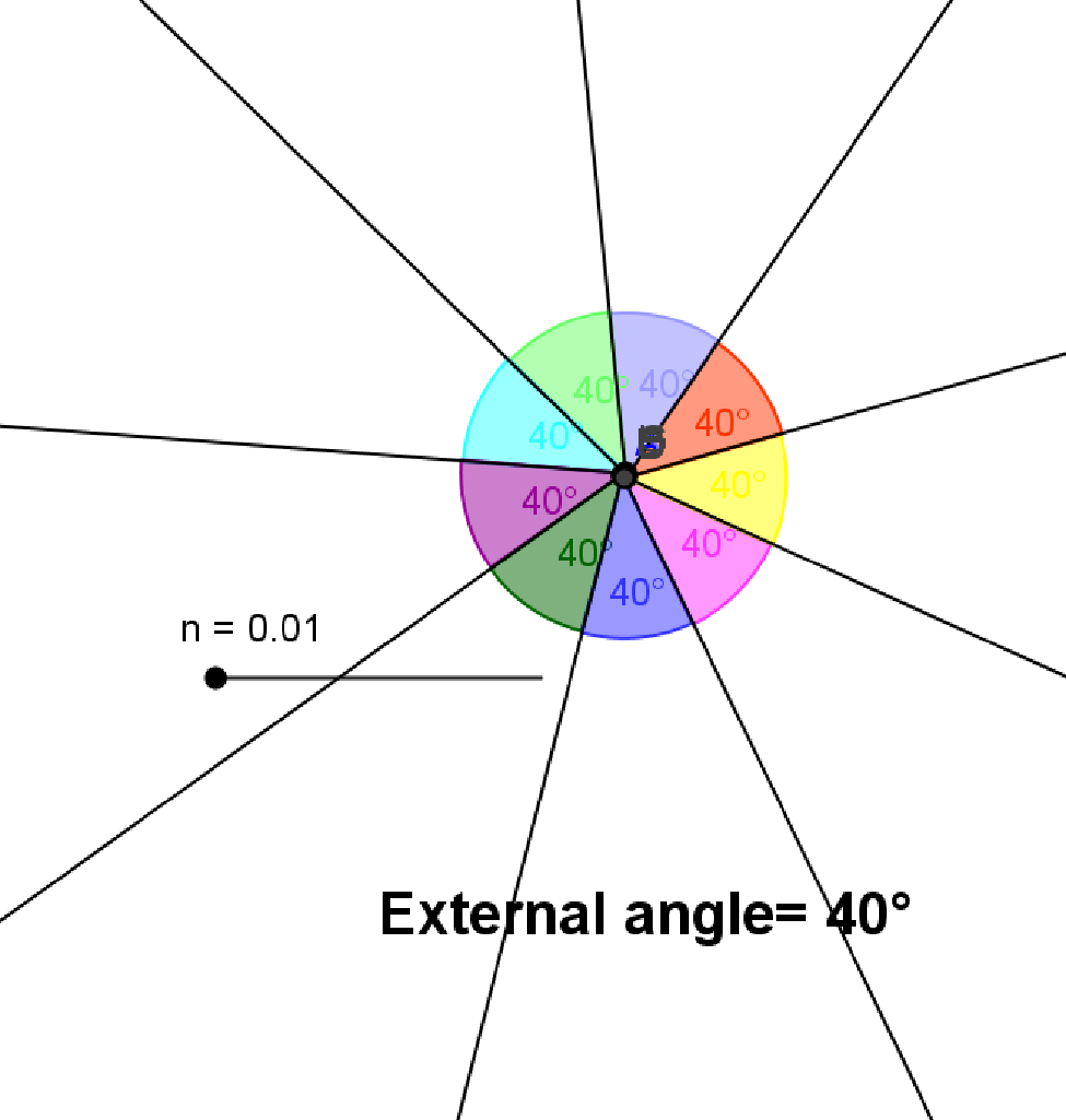
	13) In the Insert Text type "External angle= " + α to get the Dynamic Text: Exterior Angle 400.
	14) Drag the slider to change the size of the polygon, observe that each angle remains 400. Drag the slider to reduce value of n, what happens when n is very small, n=0.01? What can you conclude from this?

Exploring the effect of a, b and c on graph of quadratic f(x) = ax2+bx+c

Instructions

	1) Open a new GeoGebra file.
	2) Show the algebra window , input field and coordinate axes (View menu)
	3) Create the variable a = 1 in the Input bar. To display number as a slider in the graphics window you need to right  click the variable in the algebra window and select Show object
	4) Create a slider b using the Slider tool. Hint: Activate the tool and click on the drawing pad. Use the default settings and click Apply.
	5) As above create a slider c using the Slider tool.
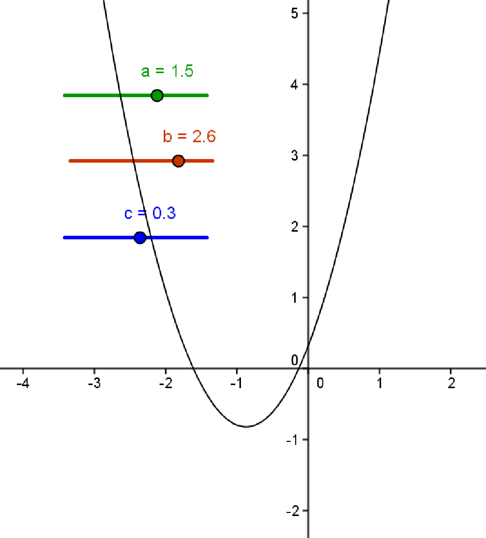
	6) In the Input bar enter f(x)= a*x^2+b*x+c
	7) To plot vertex , in Input bar Enter, A= (
	8)Select -Check box to show/hide object (in the drop down menu of slider tool)
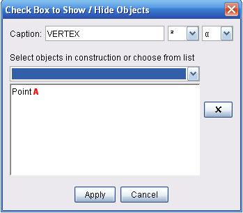	9) Click anywhere on the Drawing Pad and enter Caption- VERTEX and select point A.

Tracing the Graphs of Trigonometric Functions

Instructions

	1)   Open GeoGebra. First, we will create a point that will be the center of our unit circle. To create point A in the origin, type A = (0,0) in the input box and press the ENTER key.
	2) Next, we construct a circle with center A and radius 1. To do this, type circle[A,1] in the input box and press the ENTER key.
	3) We fix point A to prevent it from being accidentally moved. To fix the position of point A, right click point A, then click Object Properties from the context menu.  This will display the Properties dialog box shown in Figure 2. Figure 2 – The Properties dialog box.
	4) In Basic tab of the Object Properties dialog box, click the Fix Object check box to check it, then click the Close button.
	5) To construct point B at (1,0), type B = (1,0).
	6) Fix the location of point B (refer to steps 3-4).
	7) To construct point C on the circumference of the circle, click the Point tool and click the circumference of the circle.  Your figure should look like Figure 3.
	Figure 3 – The unit circle with points B and C on its circumference.
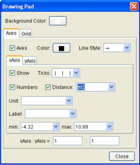
	8) We will change the interval of the x-axis from 1 to π/2. To do this, click the Options menu from the menu bar, and choose Drawing Pad from the list do display the Drawing pad dialog box shown in Figure 4. In the Axes tab dialog box, click the x-Axis tab. Click the Distance checkbox to check it and choose π/2 from the Distance drop-down list box. Figure 4 – The Drawing Pad dialog box.
	9) Now we create arc BC of circle with center A starting from B and going counterclockwise to C.  To do this, type circularArc[A, B, C].
	10) Right click the arc BC, you will see a dialog box as shown in Figure 5. Choose Arc d (or whatever is the name of your arc), then click Properties to reveal the Properties window.
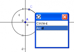
	Figure 5 – The dialog box that appears when you right click overlapping objects.
	11) In the Properties window, choose the Basic tab, be sure that the Show label check box is checked and choose Value from the drop-down list box. This will display the length of arc BC.
	12) Next, we change the color of the arc to make it visible. Click the Color tab and choose red (or any color you want) from the color palette.
	13) Click the Style tab, then adjust the Line Thickness to 5, then click the Close button. Your drawing should look like the one shown in Figure 6. Figure 6
	14)  Next, to construct the point that will trace the sine wave, we construct an ordered pair (d,y(C)) where d is the arc length and the y(C) y-coordinate (or sine) of point C. To do this, type P = (d,y(C)).
	15) To trace the path point P, right click point P and click Trace on from the context menu. Move point C along the circumference of the circle and see the path of P.
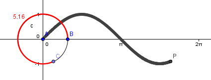
	Figure 7 - The appearance of the drawing after step 17.
	16) To create point Q that will trace the cosine wave, type Q = (d,x(C)).
	17) Activate the trace of point Q (see Step 17). Now, move point C along the circumference of the circle and observe the path of point Q.

* * * * * * * * * * *